Saving Curve

The saving curve is a diagrammatic depiction of the saving function. It shows the amount of saving at various levels of income. As he has been said earlier, the gap between the 45o line and the consumption curve shows the amount of saving at various levels of income. We can show this saving income relationship.

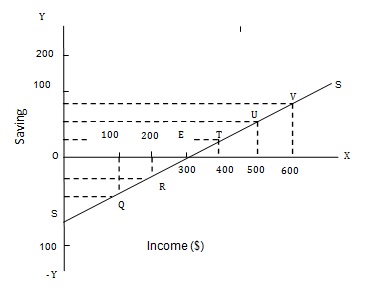
In this Fig, Income is measured on the X-axis (OX) and saving are shown on the Y-axis (OY). The Y-axis has two parts, one from O to Y which measures the positive saving and the other extends from O to Y downwards showing the negative saving or dissaving.

Now, as shown in the Fig. at an income of $300 saving are zero. The point O on the OY-axis shows the zero saving level, while point E on the OX-axis shows the income of $300. Point E showing the saving income relationship at an income level of $300 thus lies on the X-axis. As the income goes up to $400 there is a positive saving of $20. This is shown by point T. Similarly, points U and V show the saving of $40 and $60 at the income levels of $500 and $600 respectively.

On the other hand, when income is $200, the consumption is $220 and therefore there is dissaving of $20. This negative saving is shown on the AY-axis. .To plot this point, we draw a line downwards from an income level of $200 as shown on the X-axis. Then from the Y-axis, from a distance measuring $20. We draw a horizontal line parallel to the X-axis. These two lines intersect on the point R. Thus, R is the point which shown the negative saving of $20 at the income level of $200. Similarly, we plot the point Q which shown a negative saving $40 at the income level of $100. By joining these points QRETUV, we get the saving curve SS, which shows the amount of saving at various levels of income. When we extend this curve backward to meet the Y-axis the intercept OS shows the amount of dissaving that shall take place at zero level of income. In other words, when income is zero, some consumption expenditure is bound to take place, which will result in negative saving of OS.

As is clear from the above diagram, the saving curve SS lies below the X-axis for income levels ranging from O to E. This shows that at lower levels of income, saving are negative. At the income of OE, saving the zero, and for the income levels beyond E the saving become positive and keep on increasing at successively higher levels of income.

The point E on the consumption curve CC shows that level of income where consumption is just equal to income is neither more nor less. So, at this level of income savings are zero, The point E on the saving curve SS shows the level of income which correspond to zero level of savings. Before the point E, saving are negative and beyond it. saving are positive. This point where consumption is just equal to the income and hence where saving are zero, is known as break-even point.